What is the Normal Model?

Introduction

The Normal Distribution describes a symmetrical, unskewed, bell-shaped set of data around the mean, where values closer to the mean are more likely to occur than values further from the mean.

It has two parameters: The mean, representing the center, and the standard deviation. Interestingly, the mean and median are equal.

We use the normal distribution to find the probability that a random variable is less than or equal than a certain value. For example, you may want to answer the question “What percent of men are shorter than 5’11?” The normal model would be the tool to use for this.

Intuition

The Normal Distribution is impressive because it comes up everywhere. If you see a distribution that looks like this, it’s probably normal or nearly normal.

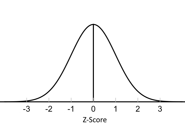
Remember back to the 68-95-99.7 rule. The space between Z = -1 and Z = 1 contains 68% of the data, (-2, 2) contains 95%, and (-3 , 3) contains 99.7%. Whenever something like that comes into play, it’s a normal distribution or a model close enough to it.

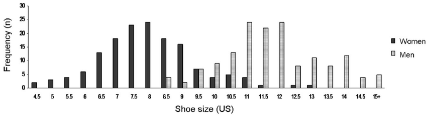
Let’s take an example you may not expect to be normal: Shoe Size.

This is bimodal, but within men and women shoe size is remarkably close to a normal distribution. You will notice that the X-axis has switched from Z-scores to size. Z-score is a unitless variable that you can use to compare almost any two instances in a normal model. You can discuss if a dog’s weight is more extreme than an earthquake’s magnitude. It tells you only what percent of the data is less than it, regardless of the model.

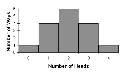
This, again, has the same iconic bell curve shape you find in the Normal Distribution. It’s strange how they line up with each other despite seeming totally different. The normal distribution has some amazing properties.

The Math Behind the Normal Distribution

There’s three steps to going from a normal model to a probability.

• First, set up a normal model with the mean(μ) and standard deviation(σ), and find the value of x you want to find the Z-score for
• Secondly, set up the fraction Z = (x - μ) / σ

• Finally, take your Z-score to a Z-table and find the corresponding probability of a Z-score equal to or lesser than it

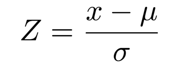
What this does, intuitively, is find the difference between your value and the mean, and then divides it by how much values tend to vary around the mean. This means that the normal distribution is normalized. You can compare one Z-Score from one normal model to another Z-Score from another normal model and know which one is more extreme or more above average. The Z-Score tells you where on the normal distribution you are, without telling you what your specific normal distribution looks like.

Reading a Z-Table

Usually, we want the probability of getting a value the same as or less than a value rather than the number of standard deviations from the mean it is. The math for this is extremely cumbersome (Look up the Gaussian Integral if you’d like to see some of it), so instead we use a Z-Table, that lists out the probabilities of a Z-score less than each Z-score.

To read a Z-table, you take your Z-Score, find the Ones and Tenths Place on the leftmost column, the hundredths place on the top row, and go to the place where they intersect.

This makes more sense with an example. Let’s take Z = 2.73. Open up your Z-table of choice, select 2.7 in the left column, and 0.03 in the top row.

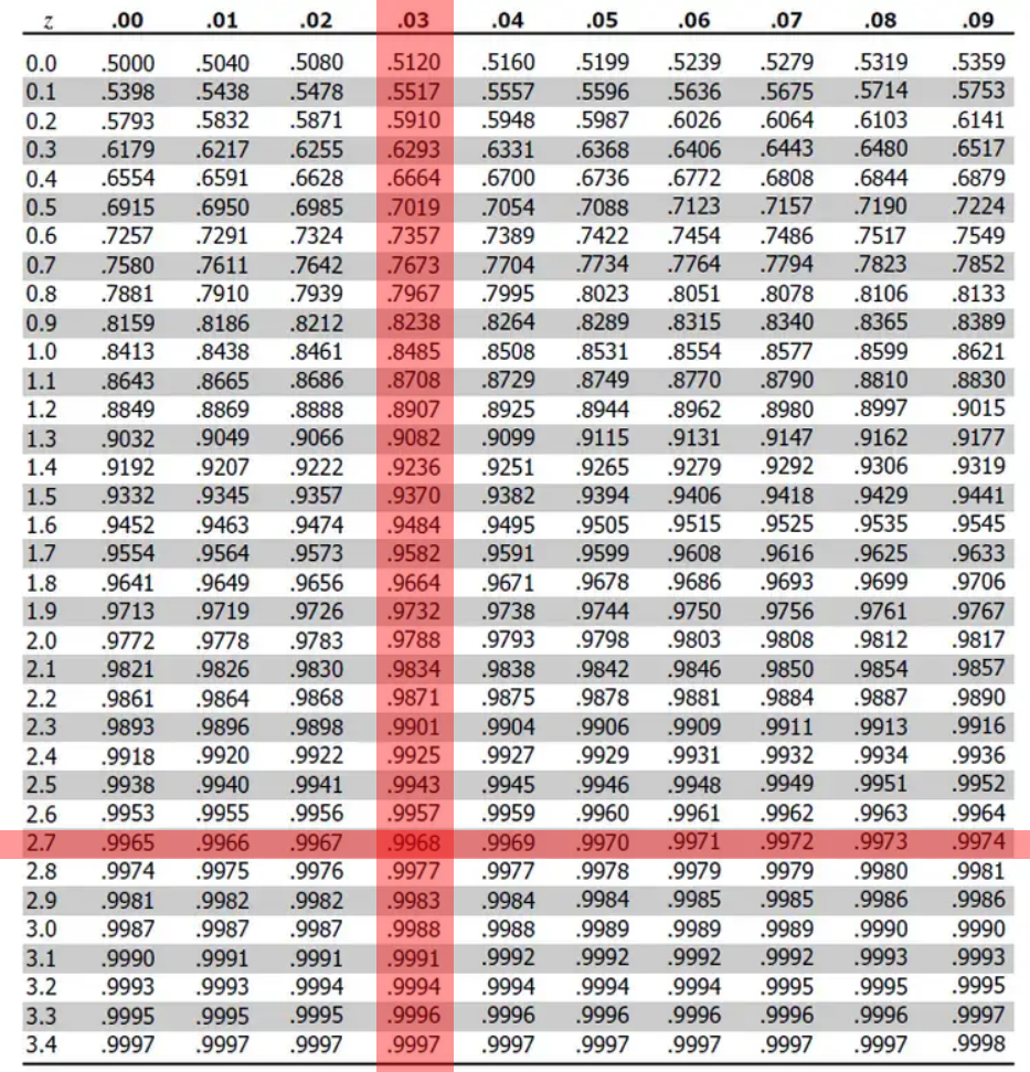
Finding the place where these two intersect on the table, we see the probability of a Z-Score under 2.73 is .9968, or 99.68%. This gets significantly easier the more you do it.

Some Examples

Imagine you have to catch a train, that comes at 9:00, and has a standard deviation of departure time of 6 minutes. Due to a broken escalator, you arrive 3 minutes late. What is the chance you make your train?

Some things to note From this:

First, this is a normal model with a mean of 9:00 and a standard deviation of 6.

Second, we arrive at 9:03

Third, we’re looking for the chance that our arrival time is GREATER than the train’s departure time. Remember that the normal distribution tells you the odds that a random variable is LESS than a certain amount.

Now, we have everything we need. The first thing to do is to find a Z-Score.

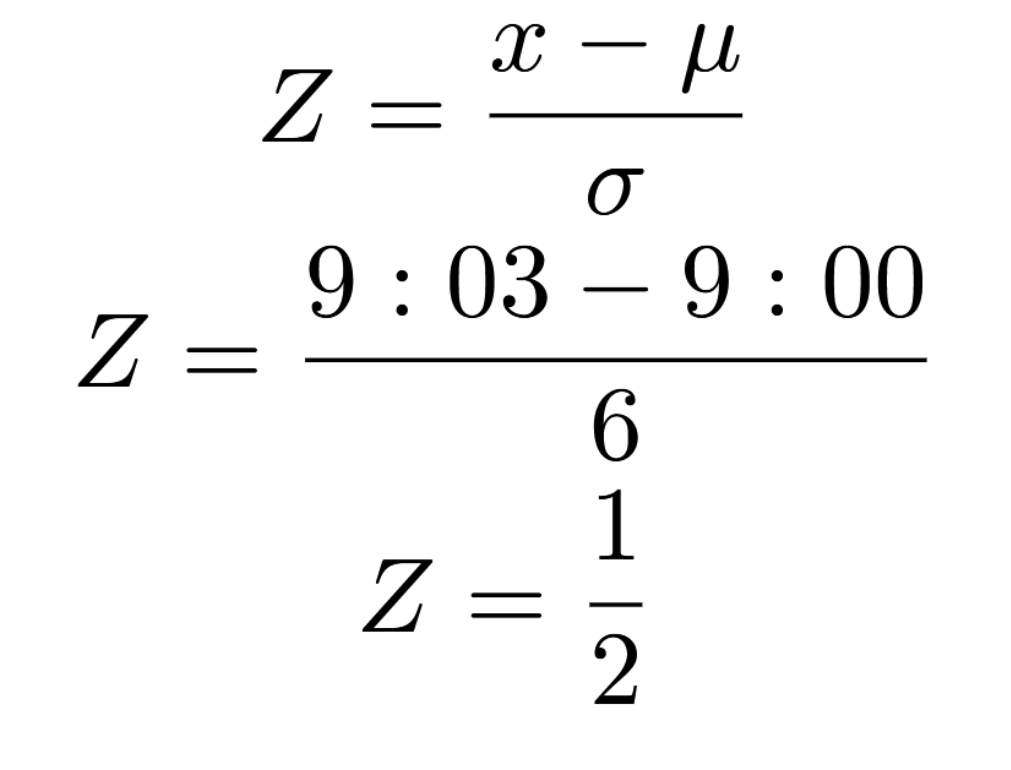
Remember that 0.5 is just a Z-Score. It’s not a probability, and other than comparisons, there’s very little we can do with this. We need to find the probability of a Z-Score under 0.5, and that’s what the Z-Table is for.

Find the ones and tenths place in the left column, and the hundredths place in the top row.

This is where the magic happens. We have converted a Z-Score, which is an unintuitive and opaque number with no clear day-to-day meaning, into the probability that the train departs before 9:03, getting .6915, or 69.15%. Now, we just have to find the probability it departs after 9:03 to get the probability we make our train.

To do this, you can just use the compliment rule, subtract the prior probability from 1, and find the odds are 0.3085%, or 30.85%. That’s it!

Hope this was of some use. If you have any other questions, comments, or concerns, feel free to contact me.

Citations

Contact

I've enjoyed putting together this website. Full credit to the Monospace Web, who created the template used for this.

If you'd like to contact me, my information is below

Brendan Heaney, Binghamton University Class of 2027

Personal Email: brendantheaney@gmail.com

University Email: bheaney@binghamton.edu

My LinkedIn

Homepage